
Microsoft Excel is the most popular spreadsheet software in the world. This versatile tool can perform calculations, manipulate text-based data, create charts and graphs, and many more. But today I discuss How to freeze cells, rows, and columns in Microsoft Excel.
Sometimes it becomes fuzzy to work with sheets when data becomes too large to be handled. One of the amazing solutions that excel provides us is “freeze cells” or “freeze panes” feature. In this blog post, we will briefly discuss “freezing cells” in Excel.
Step-By-Step guide on How to freeze cells, rows and columns in MS Excel
When you work on a large worksheet, the first row generally would not be visible when you scroll down, the same the first column wouldn’t be visible when you scroll to the right side of the sheet.
Freezing Cells feature in Excel allows a user to lock the particular rows or columns into their place, so when the user will scroll to right, left, up and down in the worksheet those selected cells will be visible all along the scrolling.
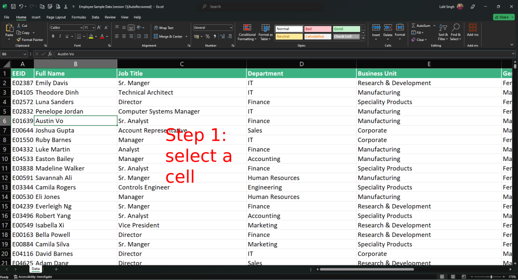
Step 1. Select the cells, rows, or columns to freeze
Firstly, click on the cell or select a group of cells, or select any particular row to freeze, so it can be visible all the time when you scroll.
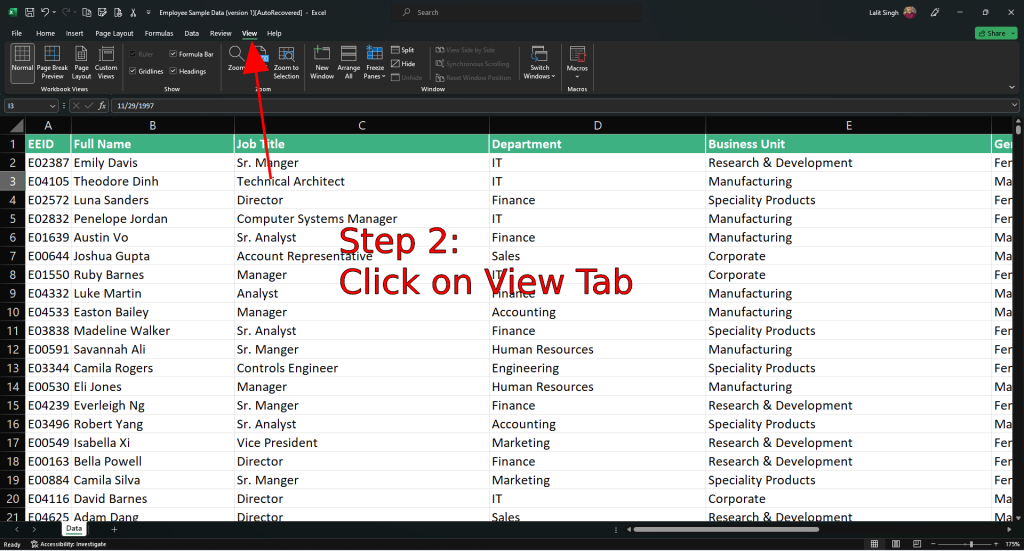
Step 2. Go to the “View” Tab
Now click on the “View” Tab on the Excel ribbon. See the below image for reference.
Step 3. Click on the “Freeze Panes” dropdown
In view tab, you will see the “Freeze Panes” dropdown in windows group. Click on the dropdown option.

Step 4. Select the Freeze option
Now you will be able to see 3 options:
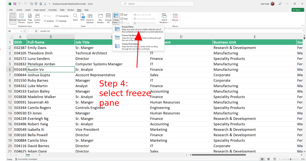
- Freeze Panes:This option freezes the above row and left of the column of your selected cell.
- Freeze Top Row:Selecting this option, the first row is going to be frozen, and you will be able to scroll over the rest of the sheet.
- Freeze First Column: This option freezes the first column while enabling scrolling through the rest of the sheet.
Select the option that you need in your worksheet. You can be able to scroll through the sheet while the frozen rows and columns or cells will remain visible.
Using Freeze Panes in Excel
Imagine you selected a single cell in the sheet and selected the “Freeze Panes” option from the dropdown. Refer to the attached video below. Now, the rows above the selected cell and the left side column will be frozen.
Freezing the Top Row in Excel Worksheet
If you want to freeze the top row of the worksheet; you have to select the second option from the “Freeze Panes” dropdown menu.
Freezing the First Column in Excel Worksheet
If you want to freeze the first column, choose the “Freeze First Column” option from the “Freeze Panes” dropdown menu. This will freeze the first column while you scroll through the sheet.
Unfreezing Cells, Rows, or columns in MS Excel:
Now if you want to unfreeze the cells, rows, or columns as we previously demonstrated, simply go to the “Freeze Panes” dropdown menu and select “Unfreeze Panes”. This action will remove all the freeze panes applied to the sheet.
Freezing cells is an amazing and useful feature in MS Excel that boosts up the productivity and view of the sheet when working with a large worksheet.